Near–infrared (NIR) Spectroscopy

The region is sub–divided into two regions: 780 to 1100 nm and 1100 to 2500 nm, the first of which is named the Herschel region. Though discovered some 200 years ago, it is only in the past 30 years that its analytical potential has been exploited. For the qualitative analysis of solid samples, invariably NIR spectra are measured by reflectance. Spectra are often complex with many overlapping peaks (Fig. 1A).

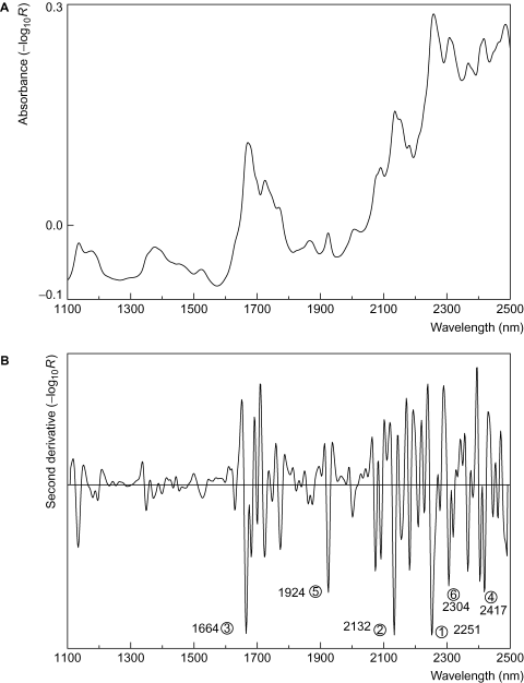
As a result of this, the technique was viewed originally with some scepticism, until the advent of modern computerised NIR instrumentation. Though the reflectance spectrum of a material is complex, its second–derivative spectrum is very suitable for identification purposes (Fig.1B).

NIR spectra are associated with molecular vibrations and consequently provide information similar to that obtained by mid-IR spectrophotometry. While NIR spectra are much more difficult to interpret than mid-IR spectra, it is their fingerprint nature that makes the technique useful for identification purposes.

NIR spectroscopy is neither a trace analytical technique nor generally suited to the identification of individual substances in multicomponent mixtures. Its strength lies in its ability to identify relatively pure samples rapidly or to identify a matrix of nearly fixed composition, such as tablets. Although it used for the quantitative assay of solids in the pharmaceutical industry, to set up a calibration model is usually a time consuming and expensive process that precludes its use for ‘one–off’ quantitative determinations. Spectra are particularly simple to measure, the technique is non–destructive and generally requires no sample preparation. A further advantage of NIR spectra is that they contain information about the physical properties of the sample, such as particle size, compaction density, poymorphs, etc., which often makes it possible to differentiate between samples of the same chemical identity, but of different grades or from different sources.

NIR absorbances correspond to overtones and combinations of molecular vibrations that have their fundamentals in the mid-IR region of the spectrum. Fig.2 illustrates the potential energy curve for a simple diatomic molecule.

The allowed energy levels, E, for such an anharmonic oscillator are given by:

Where h is Planck’s constant, v the vibrational quantum number, f the equilibrium frequency of oscillation and x the anharmonicity constant. The vibrational quantum number may take values 0, 1, 2, … . The selection rules for an anharmonic oscillator are Δv= ±1, ±2, ±3, …, and consequently transitions such as v_1←0, v_2←0,v_3←0, v_2←1, etc., are allowed (in practice, only transitions starting at v=0 are important for spectra measured at room temperature). These transitions are referred to as the fundamental frequency of vibration, first overtone, second overtone, etc., respectively. As the anharmonicity constant is typically small (x < 0.05), these spectroscopic transitions occur approximately at frequencies close to f, 2f and 3f, etc.

For most molecular vibrations the fundamental frequency of vibration occurs in the mid-IR region of the spectrum; however, the overtones occur in the NIR region, which is the basis of NIR spectroscopy.

Polyatomic molecules may exhibit simultaneous changes in the energies of two or more vibrational modes: the frequency observed will be the sum (f₁ + f₂, 2f₁ + f₂, etc.) or the difference (f₁–f₂, 2f₁–f₂, etc.) between the individual frequencies (note, 2f represents the first overtone and the subscripts 1 and 2 refer to different vibrational modes). This results in very weak bands called combination and subtraction bands – the latter are possible, but rarely observed in spectra measured at room temperature. Combination bands have a very low probability of occurrence unless they arise from two vibrations that involve a common atom or arise from bonds connected through multiple chemical bonds. The transition probabilities for overtones and combination bands are 10 to 1000 times smaller than those for the fundamental frequency and, consequently, such absorbances are weak. This weakness of absorbances can be put to good advantage in that samples may be measured without any need for sample dilution or preparation.

Sommaire

Reflectance and transmission

NIR spectra may be measured by either reflectance, R, or transmission, T. Reflectance is the ratio of the intensity of radiation reflected by the sample, I_r, to the intensity of the radiation impinging on it, I_o, hence R = I_r/I_o.

Similarly, transmission is the ratio of the intensity of radiation that passes through the sample, I_t, to that impinging on it, I_o, and hence T = I_t/I_o.

Reflected radiation is made up of two main components – specular and diffuse radiation. Specular reflection is radiation that is simply reflected directly from the surface of the sample and contains little useful information about the sample for identification purposes.

Diffuse reflection refers to radiation that has penetrated into the particles of the sample, undergone multiple reflections within the substance and re–emerged after the various characteristic absorptions of the substance have occurred.

Fig.3 shows a schematic illustration of diffuse reflectance, I_r. Such reflected radiation gives rise to chemical information. The path length of the radiation is dependent on numerous factors, such as particle size, particle shape and sample compaction, and therefore also contains information about the physical state of the sample. The exact path taken by the radiation is difficult to describe mathematically and consequently there is no totally satisfactory theory for diffuse reflectance. However, the Kubelka–Munk theory is a useful approximation for NIR reflectance measurements.

The Kubelka–Munk function, f(R_a), relates the absolute reflectance, R_a, of the sample to its absorption coefficient, k, and scattering coefficient, s, according to:

The absorption coefficient is equal to the absorptivity, a (as defined by the Beer–Lambert law), multiplied by the concentration, c, and hence the Kubelka–Munk function is related to concentration according to:

Practical reflectance measurements are made with respect to some standard reflecting material. A measure of practically measured reflectance (R_m, although R is commonly used for this function) is the ratio of the intensity of light reflected from the sample to that reflected from a background or reference surface. The dependence of reflectance with concentration is often no better described by the Kubelka–Munk function than by using the apparent absorbance (A = –log₁₀R) and Beer’s law:

where a′ is a proportionality constant.

The passage of radiation through a solid or powdered sample occurs by what is termed diffuse transmission. The radiation undergoes many internal reflections within the particles of the sample and emerges in all directions (Fig.3).

The transmission of a 2 to 5 mm thickness of compact powder (e.g. a tablet) when measured with respect to air will typically be 10^–4 to 10^–6. Useful transmission measurements are commonly limited to the wavelength region below 1900 nm, and are not particularly good for identification purposes.

Instrumentation

Spectrometers that record NIR spectra are generally based on filter, grating or interferometer designs. Instrumentation is similar to that used for ultraviolet and/or visible absorption spectroscopy and based on fixed wavelengths, scanning or diode array systems. Tungsten–halogen lamps serve as energy sources, while lead sulfide and/or indium gallium arsenide detectors are used. Present–day instruments are computer controlled, which enables spectra to be measured in a matter of seconds and saved to a computer file.

A typical spectral file for a grating instrument consists of 700 data points at 2 nm intervals over the wavelength range 1100 to 2498 nm. Fourier transform (FT) instruments normally give outputs in wavenumbers and a typical file has 500 data points at 12 cm^–1 intervals over the range 4008 to 9996 cm^–1 (i.e. 2495 to 1004 nm). Saved spectra are generally the average of a number of scans so as to reduce noise levels. Measurements are made by reflectance or transmission.

Data processing and presentation of results

Though the original NIR reflectance spectrum of a substance is complex and often relatively featureless, its second–derivative spectrum is very suitable for identification purposes. Taking the second derivative of the spectrum largely removes the effects of baseline offsets and baseline slopes. This is illustrated in Fig. 4A, which shows a spectral absorption peak with:

1.   horizontal background
2.   linearly sloping background
3.   a curved background plus zero offset.

Taking the first derivative with respect to wavelength removes any offset and reduces a linearly sloping background to a simple offset (Fig. 4B). Taking a further derivative (i.e. second derivative) removes this offset and all three spectra are now almost identical (Fig. 4C).

The positions of the negative peaks in the second–derivative spectrum correspond to the positions of peaks in the original spectrum. This can be seen for acetomenaphthone in Fig. 1A and Fig.1B. Derivative spectra can be calculated by a variety of methods. The simplest is to calculate the difference between blocks of data points on either side of the wavelength at which the derivative is required. This point is replaced by the difference between the two blocks (Fig.5).

The process is repeated across the whole spectrum, moving along one data point each time. To calculate a second derivative, etc., the process is simply repeated the required number of times. By suitable selection of the number of data points in the sample block (ss) and the number of points in the gap block (gs), the degree of spectral smoothing can be adjusted. Values of ss = 3 to 10 and gs = 0 are commonly used. Sample spectra and reference spectra must be treated equally.

Another commonly used method is that of Savitzky and Golay (1964). In effect, a polynomial of specified order is fitted by least squares to the data using a specified number of data points before and after the point at which the derivative is required. The estimated derivative is then the derivative of the resultant fitted polynomial. The process is repeated across the whole spectrum, moving one data point each time. This many least–squares fits could be laborious and time consuming. However, provided the data points are all equally spaced, they can be achieved very efficiently using a Savitzky–Golay filter. Typical parameters used are 3 to 10 data points with a polynomial fitting order of 2 to 4. The Savitzky–Golay method has the advantages that it is a published method and gives more control over the smoothing parameters (number of data points and order of polynomial).

Sample compaction and changes in particle size of samples can have a pronounced effect upon the spectrum of a sample. Fig. 23.6A shows spectra for samples of lactose monohydrate of different particle sizes.

If it is required to reduce such effects, there are various data pretreatments that may be applied. The best one for a particular application is usually found by trial and error. The standard normal variate (SNV) transformation is one of several normalisation processes that may be used. The ordinate (absorbance, second–derivative absorbance, etc.) of a spectrum at each wavelength, i, is replaced by z_i according to:

where ȳ is the mean spectral value over the complete spectrum, s is the standard deviation of the spectral values over the complete spectrum and y_i is the spectral value at wavelengthi. Fig.6B shows the lactose monohydrate spectra after SNV transformation, which demonstrates that most of the effects of particle size have been removed.

Multiplicative scatter correction (MSC) is another commonly applied transformation used to minimise light–scattering effects. For each spectrum in a set (e.g. calibration set) a linear regression of the ordinate values on those for the mean spectrum of the set is performed. The intercept, a, and slope, b, are then used to generate a new spectrum according to:

where y_i is the original ordinate value at wavelength i and y_MSC,i is the corresponding corrected value. In effect, each spectrum is adjusted so that it fits the mean spectrum as closely as possible. Unlike the SNV transformation, the mean spectrum must be stored so that the same transformation may be applied to the spectra of test samples. An advantage with respect to SNV, however, is that the corrected spectra have an ordinate scale similar to that of the original spectra.

Systems suitability test

Most NIR instrument and/or software systems prevent sample measurements being taken until a systems suitability test has been run. Checks typically include photometric noise, wavelength accuracy, band–pass, etc., and are normally carried out once per day. The European Pharmacopoeia (2002) provides a number of guidelines for performance checking, as also does the Pharmaceutical Analytical Sciences Group. A number of independent tests for noise and wavelength accuracy, etc., can be carried out easily.

Standard reference materials (SRMs) are available from the United States’National Institute for Standards and Technology (NIST) for wavelength accuracy measurements. Most instrument manufacturers can also supply standards that are traceable to the NIST standards. The reflectance spectrum of an equal mixture by mass of dysprosium, erbium and holmium oxides is used as a standard and exhibits 37 reflectance minima in the NIR wavelength range (Weidner et al. 1986). Fig.7A shows the reflectance spectrum of a mixed lanthanide oxides standard over the wavelength range 1100 to 2500 nm, with the major minima marked. The reference wavelength values are slightly band–pass dependent and the values shown are for an instrument with a band pass of 10 nm. The reference values given by NIST have an uncertainty of ±1 nm. As some minima are associated with a sloping background it is important to display the spectrum in terms of reflectance rather than absorbance (–log₁₀R), this being the condition under which NIST documented the wavelength values. Pure (>99.99%) samples of the lanthanide oxides are readily available and may be used instead of expensive NIST wavelength SRMs. Examples of reflectance spectra obtained for the three separate oxides measured on a FT-NIR instrument are shown in Fig.7B. As the band pass of a FT-NIR instrument varies in terms of wavelength across the spectrum, care is needed in selecting the reference values. In Fig.7B, reference values for a 10 nm band pass were used in the range 4000 to 7000 cm^–1 and 5 nm band–pass values for above 7000 cm^–1. A typical commercial grating instrument (data stored at 2 nm intervals) might have a wavelength accuracy of ±0.3 nm, while an FT instrument (data stored at 12 cm^–1 interval) has an accuracy of ±2 cm^–1. Some form of wavelength interpolation between stored data points is essential when locating the position of minima (see section Wavelength repeatability).

NIST and NIST traceable wavelength standards for transmission measurements are also available; however, an inexpensive alternative is to use trichloromethane, which exhibits sharp absorption peaks at 1152.1, 1410.2, 1619.9 and 1861.2 nm (Busch et al. 2000).

Wavelength repeatability can be checked by recording a sample spectrum a number of times (e.g. >12, without moving the sample between scans) and calculating the standard deviation of the wavelengths of minima in the second–derivative absorbance spectra. Materials with well–defined narrow second–derivative peaks, such as the mixed lanthanide oxides wavelength standard (suitable for wavelengths below 2200 nm) are ideal. Alternatively, compounds such as ascorbic acid, aspartame, benzoic acid, salicylic acid and sucrose, may be used. Some form of wavelength interpolation between stored data points is essential when locating the position of minima. Fitting a quadratic curve to three consecutive data points that encompass a minimum and calculating the exact position of the minimum from the equation works well. Let the fitted equation be A=a+bλ+cλ², where A is the second–derivative absorbance, a, b and c are the fitted coefficients; then λ_min=−b/2c. Typical standard deviations for peak wavelengths are <0.01 nm for a grating instrument that stores data points at 2 nm intervals and <0.5 cm^–1 for a FT instrument that stores data at 12 cm^–1 intervals.

This can be determined by measuring the absorbance of a single sample a number of times (e.g. >12) and calculating the standard deviation at each wavelength. To obtain an estimate of the instrument noise, as distinct from the repeatability of sample measurements, the sample should not be moved between scans. To reduce the effects of wavelength repeatability errors, the sample used should ideally have a flat spectral response. Rapid repeat scanning of a sample can result in sample heating and introduce unwanted variations in the spectra. For this reason sintered perhalopolyethylene cake and/or carbon black reflectance standards are not recommended for this test. The noise level should be checked over the full wavelength range of the instrument and for both low and high absorbances. For low–absorbance samples the instrument reference standard, barium sulfate and titanium dioxide, are ideal. As strong absorbers, substances such as carbon black, finely ground sucrose and butylated hydroxytoluene, may be used. Though far from spectrally flat, the mixed lanthanide oxides wavelength standard is thermally stable and works well. Noise levels depend upon the number of primary scans averaged. However, under normal recommended operating conditions, the noise level is generally very low and differences between repeat spectra are not easily visible without expanding the display scale. For typical grating instruments, repeat measurements can be expected to give a standard deviation of <0.05 milli–absorbance units (mAU) across the wavelength range 1100 to 2500 nm and absorbance range zero to unity. The noise level for a typical FT-NIR instrument would be <0.5 mAU.

All reflectance measurements made using a sample stage include specular radiation from the sample stage itself and from the sample bottle (Fig. 23.8A and Fig. 23.8B). The effect of this is to make a plot of measured absorbance (–log₁₀R_m) versus true (absolute) absorbance (–log₁₀R_a) curved and hence limit the photometric range. To check photometric linearity, and measure the extent of specular radiation, samples of known absolute reflectance are required. Suitable standards with absolute reflectances of 0.02 to 0.99 are available from NIST and various instrument manufacturers. The standards typically are carefully prepared mixtures of sintered perhalopolyethylene cake and carbon black and should be regularly sent for re–certification. Tables of actual reflectance versus wavelength are provided for each standard. The measured reflectance for a given standard (relative to the instrument standard) can be expressed as follows:

A plot of R_m versus R_a at a given wavelength should therefore give a straight line if the photometric response is linear. However, in practice, a small degree of curvature is usually observed. The value of k′ represents the specular and/or stray radiation expressed as a fraction of radiation reflected by the instrument reflectance standard. Values for k′ vary from one instrument to another and change with time as the surface conditions of the sample stage, etc., age (k′ < 0.01 is typical). Measuring the signal without a sample on the stage also gives a simple method of accessing the background specular and/or stray radiation, provided external light and internally reflected radiation can be avoided. Similarly, measuring an empty bottle (no top) gives a measure of I_s + I_ss relative to the instrument standard.

NIR spectra can be measured by either reflectance or transmission. Reflectance measurements are particularly easy to make. Common glasses (borosilicate, soda, etc.) are virtually transparent to NIR radiation and powdered samples may be measured in such sample bottles directly (Fig.9A and Fig.9B).

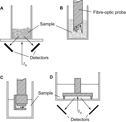
The radiation reflected by the sample is measured as a function of wavelength and with respect to the reflectance of a suitable standard, such as a flat disc of a ceramic or Spectralon. Spectra are clearly dependent upon the reference chosen and the reproducibility of such standards can be a problem when it comes to transferability of spectra from one instrument to another. This problem has not been completely resolved at present. Fibre–optic probes that can be inserted directly into the sample can be attached to many instruments (Fig.9B). Liquids can be measured using conventional cuvettes or by transflectance, again using a fibre–optic probe fitted with a transflectance tip (Fig.9C), or directly on a sample stage in a cup with a suitable reflector (Fig.9D). Transflectance reflectors may be gold plated, stainless steel, PTFE, etc., and constructed with various path-lengths. The optical path–length for transflectance is twice the physical path–length as the radiation passes through the sample twice. For most liquid samples an optical path–length of 1 to 5 mm is suitable.

For the measurement of powders, it has been recommended that sample bottles should be filled by ‘pouring’ the powder into the bottle without tapping (Yoon et al. 1998). Tapping causes compaction of the powder and was found to result in poor sample–measurement repeatability. For reflectance measurements, the sample thickness should be sufficient such that any further increase in sample thickness has no effect upon the spectrum. Typically, NIR radiation penetrates 1 to 3 mm into a powdered sample and a sample thickness of >10 mm is recommended to give an effective ‘infinite thickness’. For a compact material, such as a tablet, the reflected radiation will penetrate only 0.1 to 1 mm. The sample bottle diameter should exceed that of the radiation beam. For many instruments this means a bottle of diameter of about 10 mm or greater. Sample bottles should be chosen that have smooth bases, otherwise specular reflectance varies from one bottle to the next, as well as the orientation on the sample stage. A typical sample bottle contributes 2 to 10% of specular radiation to the reflected signal. The same type of sample bottle should be used for both test samples and reference materials.

Sample–measurement repeatability is very dependent upon the nature of the sample. Liquids and solutions are highly reproducible because of the homogeneous nature of the sample. Crystalline powders usually show poor repeatability because of varying specular reflection from the crystal surfaces. Specular reflection distorts the ‘absorbance’ spectrum and limits the usable photometric range. Identification algorithms can be affected markedly by the crystallinity of samples. Careful crushing of the material to reduce the particle size can help to minimise the effects. Vibrational patterns are affected by differences in the crystal lattice and hence different polymorphs show significant differences in their NIR spectra (Blanco et al. 1998; Patel et al. 2001).

Solvents for the preparation of solutions are somewhat limited. Only carbon tetrachloride and carbon disulfide among the common solvents are transparent throughout the entire NIR region. Methylene chloride, dioxane, heptane, acetonitrile and dimethyl sulfoxide have regions below 2200 nm that can be used.

Water has a particularly strong absorbance spectrum in the NIR region and samples must be protected from uptake or loss of water from or to the atmosphere. The presence of water can be recognised easily by the characteristic absorption peak in the range 1900 to 1940 nm. The exact peak position depends on the nature of the water – free or water of crystallisation, and the extent of hydrogen bonding. The water peak in the spectrum of lactose monohydrate (Fig.6) and the residual water in the chlortetracycline hydrochloride samples (see Fig.15) can be easily seen.

Intact tablets may be measured as easily as any other sample. A sample bottle that contains tablets randomly packed may be placed on the sample stage or single tablets may be measured directly. The depth of penetration of reflected radiation from compact materials, like tablets, is limited to only a few tenths of a mm. Markings on tablets can affect the spectra and a decision as to measure one side or both needs to be made. With coated tablets it is possible for the reflectance spectrum to be dominated by the coating material, though some radiation will penetrate into the core. Tablets can be crushed and the powder measured in a sample bottle if required.

With grating instruments, spectra commonly exhibit a small anomalous peak known as a Wood’s peak at about 1520 nm. The magnitude of the peak is dependent upon the difference in diameters of the sample and reflectance standard used: the greater the difference, the larger the peak (Fig.10). It can be quite pronounced in the spectra of poorly absorbing substances and care is required not to confuse the Wood’s peak with those from the material. Tablets, which generally have a small diameter, when measured by directly placing them on the sample stage often show a prominent Wood’s peak.

Functional groups such as X–H, where X is C, N, O and S, have a small reduced mass and hence high fundamental frequency of vibration and are particularly important for NIR spectroscopy – the first and second overtones appear in the NIR region. Groupings such as C–Cl, C–F, C=O, etc., with high reduced masses are of less importance in NIR spectroscopy as their fundamental frequencies are low and their overtones generally also appear in the mid-IR region. For organic molecules, the C–H bond is the most important and for alkanes its fundamental stretching vibration in the mid-IR region at about 2960–2850 cm^–1 gives rise to first and second overtones at approximately 1700 to 1730 and 1150 to 1170 nm in the NIR region. The C–H group stretching and deformation vibrational modes give rise to combination bands in the region 2000 to 2500 nm. Water is a particularly strong absorber in the NIR region, with the O–H first overtone of the stretching vibration occurring at 1450 nm (second and third overtones at 970 and 760 nm, respectively). Alcohols similarly show absorptions around 1450 nm. A very intense absorption occurs in the region 1900 to 1940 nm for water and has been assigned to the combination band between the fundamental stretching and deformation vibrations of the O–H bond; in the case of alcohols this vibration occurs at a somewhat longer wavelength. Temperature can have a marked effect on the spectra of compounds with hydrogen bonds. The spectrum of water is particularly sensitive to temperature, with changes in both the intensities and band positions. Similar shifts are observed for different states of adsorbed water.

While characteristic wavelengths, such as those mentioned above, can often be identified readily in the NIR spectrum of a material, the general complexity of NIR spectra precludes any easy interpretation and identifications are based on comparison with reference spectra. Fig. 11 gives a summary of the positions of some of the more important NIR absorptions. More extensive lists of NIR vibrations are given by Osborne et al. (1993) and Burns and Ciurczak (2001).

Identification of samples depends in one way or another on comparing sample spectra to spectra of known standards. Three simple classification procedures are described below.

Peak positions

In this method of identification, the sample, S, and reference, R, spectra are compared by calculating a correlation coefficient between them. If two spectra rise and fall in perfect synchronisation with one another (Fig. 23.13A), then plotting the amplitude of S against that of R at each wavelength results in a straight line (correlation plot, Fig. 23.13B).

A numerical measure of the correlation can be obtained by calculating the dot product, r_d, or product moment, r_p, correlation coefficient:

S_i and R_i are the ordinate values of the two spectra being compared at wavelength i, while S̄ and R̄ are the mean values across the selected wavelength range. The summations are performed over the selected wavelength range, which is usually the complete measured spectrum. An r value of unity represents a perfect match. However, in practice r is always less than unity because of noise. There is little to choose between these two correlation coefficients. For second–derivative spectra they give almost identical results as the mean value for a second–derivative spectrum is usually close to zero. When original absorbance (–log₁₀R) spectra are being used, the product–moment correlation coefficient often gives better discrimination. However, because of the general increase in absorbance with increase in wavelength observed for typical NIR spectra, correlation values are all very close to unity and are of little use for discrimination purposes. The product–moment correlation coefficient is less affected by data pre–treatment than the dot–product correlation coefficient, but sample and reference spectra should always be treated equally. A critical r value of 0.95 has commonly been used as a cut-off point; r values greater than 0.95 indicate a positive identification, and values below 0.95 indicate a mismatch. The exact value needs to be found by trial and error (see the section Creating a database).

Crystallinity has a marked effect on identification by correlation in wavelength space (and other identification algorithms). The relative magnitudes of peaks are very dependent upon the presence of specular radiation in the reflectance signal. Differences in crystallinity can cause r to fall to very low values and a correlation plot characteristically shows a number of intersecting straight lines rather than the ideal single line. This is illustrated for the salicylic acid sample spectra in Fig.12 in the correlation plot (Fig.14), which shows that different small wavelength regions of the spectra show good correlations (i.e. the individual lines), though the overall correlation coefficient is only 0.9 because the lines are not coincident. Careful visual inspection of spectra is vital when trying to identify substances.

Small shifts in wavelengths between sample and reference spectra can have a disastrous effect on identification by correlation. For a typical second–derivative spectrum, a shift of 1 nm might cause the correlation coefficient to fall to 0.97. This needs to be kept in mind if sample and reference spectra are measured on different instruments.

This algorithm compares spectra by testing if the sample spectrum falls within an ‘acceptance envelope’ centred on a mean reference spectrum. A representative number of samples of the reference material, which should include all acceptable variations in parameters such as particle size, crystallinity, water content and purity, are measured and the mean spectral value and standard deviation at each wavelength calculated. An acceptance envelope on either side of the mean reference spectrum is then calculated, corresponding to the standard deviation multiplied by some critical value. The amplitude of the envelope changes across the spectrum, which reflects that some regions are more variable than others (Fig.15). Spectral regions associated with water, for example, typically show greater variation. The size of the envelope (i.e. critical value) depends upon the number of reference spectra, number of wavelengths and the probability level required.

The mean, x̄_i, and standard deviation, s_i of the n reference spectra at each wavelength i are calculated:

The test is simply a two–sampled Student’s t test carried out at each wavelength over the whole spectrum or part of the spectrum of interest. Critical values of t need to be calculated according to the number of wavelengths used as well as the reference sample size. Table.2 lists the critical values for some commonly used reference sample sizes, number of wavelengths and probability levels (with less than 10 to 12 reference samples, the critical t values are unreasonably large). Further details of the method and how critical values can be calculated are given in Gemperline and Boyer (1995). A sample spectrum with a t value that exceeds the critical value (i.e. outside the acceptance envelope) is considered to have come from a different population to that which the reference spectra belong. For many purposes it is sufficient to select a critical value by trial and error.

Unlike correlation in wavelength space, this algorithm is sensitive not only to the shape of the spectrum, but also to its magnitude; therefore, some form of data pre–treatment is commonly applied before comparing spectra. The use of derivatives and/or SNV normalisation to remove unwanted base–line shifts, etc., is typical. The algorithm is very sensitive to small spectral differences and can be used not only for identification, but also to distinguish between different grades or sources of materials. The high sensitivity of the procedure makes it difficult to transfer between instruments.

There are numerous chemometric procedures that can be used for the classification of NIR spectra. Methods based on principal component analysis (PCA), such as soft independent modelling of class analogies (SIMCA) or simple visual inspection of PCA score plots, can be very useful for distinguishing between the spectra of closely related materials. Textbooks on chemometrics should be consulted for further details (Adams 1995; Martens and Næs 1991; Næs et al. 2002; Otto 1999). The tutorial review by Downey (1994) is a useful guide. The software supplied with many NIR instruments commonly includes a range of chemometric algorithms.

Creating a database

Compounds with long aliphatic chains, such as hydrocarbons, stearates and waxes, are difficult to distinguish as the spectrum becomes dominated by the –CH₂ groups. Starches and related compounds, such as maltodextrins, gums and other materials with polysaccharide groupings, are difficult to distinguish from one another reliably. With inorganic compounds, which often have little or no genuine absorbance, care is required that any apparent spectral matching is not from absorbances caused by residual moisture, Wood’s peak and/or the sample bottle itself. Mid-IR and other spectroscopic techniques are most probably no better for these problem compounds – the extremely good signal–to–noise level in NIR spectra means that often the chemometric classification techniques are able to distinguish more easily between closely related compounds than they can for other spectra.

The ability of NIR spectroscopy to detect both physical and chemical differences between samples means it can used like fingerprinting. For example, batch–to–batch variation of tablets, or tablets manufactured at different sites, can often be distinguished. Similarly, the detection of counterfeit products is possible (Scafi and Pasquini 2001). Spectra of a representative sample of the genuine product are compared to those of the suspected counterfeit. While spectral comparison methods, such as maximum wavelength distance may be used, methods such as PCA are often to be preferred. A simple visual plot (two- or three–dimensional) of the principal component scores is often sufficient. Different data pre–treatments (use of derivatives, SNV, MSC, etc.) should be investigated to remove unwanted differences in spectra. Similar samples form clusters of points on the plots, while differences in scores indicate differences in samples (Fig.16). More complex methods of classification (such as SIMCA, etc.) may be usefully applied and allow probability levels to be set.

Materials and/or products must be handled with care. Tablets, etc., often rapidly exchange moisture with the atmosphere and an apparently suspect product might simply have a different moisture content. If moisture differences are not important, then genuine and suspect samples should be allowed to equilibrate to ambient humidity before measurement. When differences in moisture are important, measurements must be made as soon as the samples are opened (e.g. tablets measured immediately they are removed from a blister pack).

Examination of the principal component loadings plots can sometimes indicate possible causes for the differences between samples, especially those with just one major cause of difference. For example, when the largest difference is due to moisture content (genuine and test samples well separated along the first principal component), the loading plot resembles the spectrum of water.

Quantitative methods of NIR analysis are generally time consuming to set up and not suited to ‘one–off’ assays. However, once developed, a quantitative assay takes little more than the time to record a sample spectrum. The purpose of calibration is to construct a model that relates the sample concentration of one or more analytes to the spectral data from training samples (those samples used to create the model) and then to use the model to predict the analyte values of future new samples. NIR is best suited to measuring major components [10 to 90% by mass (m/m)], though with strongly absorbing substances useful calibrations as low as 1% have been achieved. The strong absorption exhibited by water often allows it to be determined at <0.1% m/m levels in solvents by transmittance. Transmittance NIR spectroscopy generally gives better results for solids than reflectance, as it is less sensitive to the inhomogeneity of the sample and gives results more representative of the bulk material.

The complex nature of NIR spectra makes it unlikely that, even for simple mixtures, a unique wavelength for the analyte (unaffected by other compounds) can be found. Some form of multivariate calibration procedure, such as multiwavelength linear regression (MLR), or whole–spectrum methods, like principal component regression (PCR) and partial least–squares regression (PLSR), will be required. Details of these methods can be found in numerous textbooks (Adams 1995; Burns and Ciurczak 2001; Martens and Næs 1991; Næs et al. 2002; Otto 1999). A recent review on multivariate calibration has been written by Brereton (2000). Software provided with most spectrophotometers usually includes these calibration methods. Specialised software packages are also readily available, such as PLS-Toolbox (Eigenvector) for MATLAB (MathWorks), Pirouette (Infometrix), Unscrambler (Camo ASA) and SIMCA-P (Umetrics).

Calibration involves a number of steps:

Sample selection for constructing the model is extremely important. Methods such as PCR and PLSR are essentially statistical, and therefore it is vital that the calibration samples cover all possible sources of variation likely to be encountered in the samples that are later to be predicted. All possible chemical components and their range of concentrations, along with all variations in physical properties (e.g. particle size, powder compaction) must be included if a robust model is to be produced. Samples should be designed such that there is a minimum of correlation between all the concentrations or other properties of the components. The generation of such samples to cover a sufficiently wide range of compositions for products such as tablets, which are normally manufactured to within very tight limits, presents numerous problems. Useful guidelines are provided by the Pharmaceutical Analytical Sciences Group. Blanco et al. (2001) investigated a number of strategies to extend the composition range. Synthetic samples, prepared by mixing weighed quantities of the pure components, and doped samples, made by adding known amounts of active component or excipients to powdered production samples, may be used. Neither approach is entirely satisfactory, though sample sets that contain production, doped and synthetic samples gave acceptable models. Reference values for the analytes of interest must be measured for the samples using a reliable analytical technique, such as HPLC, UV–visible spectrophotometry or titration. The accuracy of the model can not be better than that for the reference values. The samples should be divided at random into two sets; a calibration set and a validation set (a ratio of 2 or 3 to 1 is suitable). The calibration set is used to construct the model, while the validation set is used to test the model. These two data sets must be independent; for example, samples from the same batch of a product should not appear in both sets. While there are no fixed recommendations for the number of calibration samples required (it depends upon the complexity of the samples and calibration model), a minimum of 30 is not atypical. Six to ten samples for each wavelength and/or principal component used in the model is a minimum requirement.

Before applying MLR, PCR, etc., spectra generally require some form of pre–treatment to remove baseline shifts, particle size effects, etc. Commonly applied pre–treatments are first- or second–derivative, SNV, MSC or other normalisations. Combinations of such transformations are applied often. There are no definite rules for selecting the best pre–treatment to use, apart from trial and error. Similarly, the choice of model (MLR, PCR, PLSR, etc.) is also largely a matter of trial and error until the best is found.

With simple samples, such as solutions or solids in which only a single component is variable in a nearly constant matrix, it is often possible to construct a calibration model based on MLR. The concentration, c, of the analyte is modelled to an equation of the form:

The coupling of a NIR spectrometer and scanning microscope allows spectroscopic imaging of surfaces. Not only can small samples be identified, but information about the distribution of different chemical components and their particle size can be obtained. Commercial reflectance NIR microscopy mapping systems with spectral resolution of 4 to 16 cm^–1 and spatial resolution of approximately 5 to 20 μm are available. Typically, a surface area of 1 to 10 mm² of the sample is analysed by recording a spectrum for each 20 × 20 μm² area of sample, which allows a ‘grid’ of spectral information to be constructed – this gives many thousands of spectra. Spectral information comes from the top surface layers down to a depth of approximately 30 to 100 μm and represents 10 to 100 ng of sample. By using suitable chemometrics the spectra may be processed to determine the chemical identity at each ‘grid’ position. Chemical image plots to show the distribution of the various chemical species may then be created for the whole surface. Such information is of value when comparing good and poor tablet blends, distinguishing between genuine and counterfeit materials, etc. Clarke et al. (2001) have described such a system using both NIR and Raman spectroscopic data to give a chemical image of pharmaceutical formulations.

There are no major collections of published NIR spectra. A small selection of NIR spectra is found in the Handbook of Organic Compounds, NIR, IR Raman, and UV-Vis Spectra Featuring Polymers and Surfactants (Workman 2001). The Third Edition of Infrared and Raman Characteristic Group Frequencies – Tables and Charts (Socrates 2001) has a section on NIR.